Terrains are at the heart of every Computer Game - be it Counter-Strike, Age of Empires, or even Minecraft. The virtual world that these games generate is the key to a great gaming experience. Generating terrain, manually, requires a ton of effort and hence it makes sense to auto-generate a pseudorandom terrain using some procedure. In this essay, we take a detailed look into generating pseudorandom one-dimensional terrain that is very close to real ones.

1D Terrain

A one-dimensional terrain is a bunch of heights defined at every point along the X-axis. An example of this could be seen in games like Flappy Bird, Galaxy, and many more. Such terrain could also be traced as the skylines of mountain ranges.

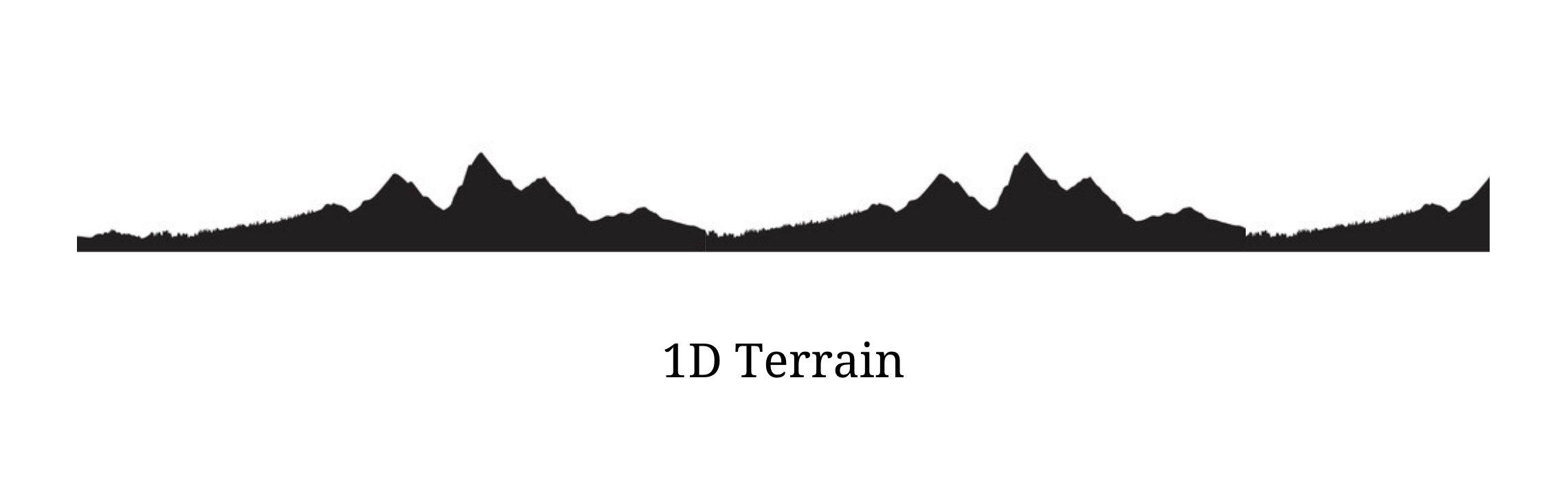
The illustration above shows a one-dimensional terrain and is taken as a sketch of a distant mountain range. The procedure we define should generate terrains as close to natural ones as possible.

Generating terrain using random values

A naive solution to generate a random terrain is by using the random function for each point along the X-axis. The random function yields random values in the interval [0, 1], and we map these values to the required height, for example [0, 100]. The 1D terrain generation algorithm using the default random function is thus defined as

import random

def mapv(v, ol, oh, nl, nh):
    """maps the value `v` from old range [ol, oh] to new range [nl, nh]
    """
    return nl + (v * ((nh - nl) / (oh - ol)))

def terrain_naive(count) -> List[float]:
    """returns the list of integers representing height at each point.
    """
    return [
        mapv(random.random(), 0, 1, 0, 100)
        for i in range(count)
    ]

The mapv function defined above comes in very handy as it helps us to map value from a source range to a target range. The terrain generation function terrain_naive takes in count as input, suggesting the number of points along the X-axis, and it returns a list of float values representing height at each of the count number of points along the terrain.

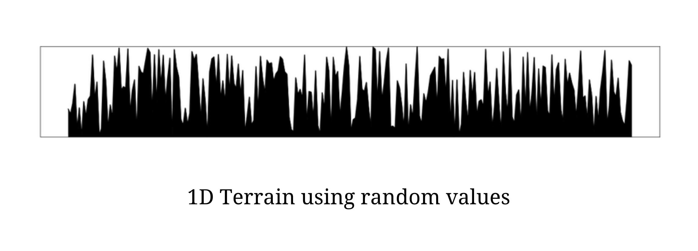
The above illustration shows the plot of the one-dimensional terrain using the above terrain_naive function. The terrain generated using this procedure has a lot of spikes and abrupt changes in height and it clearly does not mimic the terrains in the real world. Real-world terrains, although random, does not have a lot of sharp spikes, instead, the changes in height are very gradual and ensure some degree of smoothness.

In order to bring smoothness to terrain_naive generated terrains, we take a look at a famous estimation technique called interpolation which estimates intermediate values given a bunch of known points.

Interpolation

Interpolation is a method of constructing new data points within a range of a discrete set of known data points. Interpolation methods estimate the intermediate data points ensuring a “smoothened” transition from one known point to another. There are several interpolation methods but we restrict our focus to Linear and Cosine interpolation methods.

Linear Interpolation

Linear interpolation estimates the intermediate points between the known points assuming collinearity. Thus given two known points a and b, using linear interpolation, we estimate an intermediate point c at a relative distance of mu from a using the function defined below

def linp(a, b, mu):
    """returns the intermediate point between `a` and `b`
    which is `mu` factor away from `a`.
    """
    return a * (1 - mu) + b * mu

The value of the parameter mu ranges in the interval [0, 1] where 0 implies the point being estimated and interpolated is at a while 1 implies it is at the second point b.

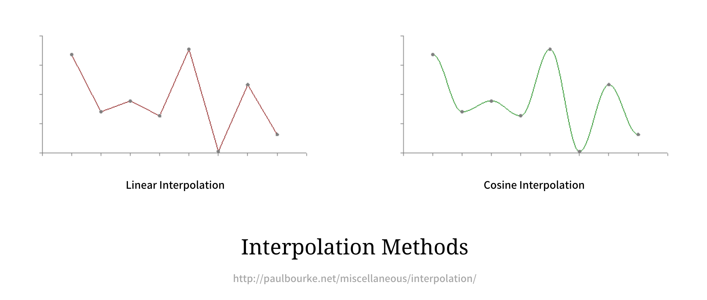
Cosine Interpolation

Linear interpolation is not always desirable as the plot sees a lot of discontinuous and sharp transitions. When the plot is expected to be smoother, it is where the Cosine Interpolation comes in handy. Instead of assuming intermediate points are collinear with the known ones, Cosine Interpolation, plots them on a cosine curve passing through the known points, providing a much smoother transition. This is could be seen in the illustration above.

import math

def cosp(a, b, mu):
    """returns the intermediate point between `a` and `b`
    which is `mu` factor away from `a`.
    """
    mu2 = (1 - math.cos(mu * math.pi)) / 2
    return a * (1 - mu2) + b * mu2

The above code snippet computes and estimates intermediate point c at a relative distance of mu from the first point a using Cosine Interpolation. Note there are other interpolation methods, but we can solve all major of our use cases using these two.

Smoothing via Interpolation

We can apply interpolation to our naively generated terrain and make transitions smoother leading to fewer spikes. In the real-world, the transitions in the terrain are gradual with peaks being widespread; we can mimic the pattern by sampling k points from the naive terrain which could become our desired peaks, and interpolate the rest of the points lying between them.

This should ideally help us reduce the sudden spikes and make the terrain look much closer to really like. A simple python code that outputs linearly interpolated terrain that samples every sample points from the naive one is as follows

def terrain_linp(naive_terrain, sample=4) -> List[float]:
    """Using naive terrain `naive_terrain` the function generates
    Linearly Interpolated terrain on sample data.
    """
    terrain = []

    # get every `sample point from the naive terrain.
    sample_points = naive_terrain[::sample]

    # for every point in sample point denoting 
    for i in range(len(sample_points)):

        # add current peak (sample point) to terrain.
        terrain.append(sample_points[i])

        # fill in `sample - 1` number of intermediary points using
        # linear interpolation.
        for j in range(sample - 1):
            # compute relative distance from the left point
            mu = (j + 1)/sample
          
            # compute interpolated point at relative distance of mu
            a = sample_points[i]
            b = sample_points[(i + 1) % len(sample_points)]
            v = linp(a, b, mu)

            # add an interpolated point to the terrain terrain.append(v)

    # return the terrain
    return terrain

The above code snippet generates intermediate points using Linear Interpolation but we can very easily change the interpolation function to Cosine Interpolation and see the effect in action. The sampling and interpolating on a naively generated terrain for different values of sample is as shown below

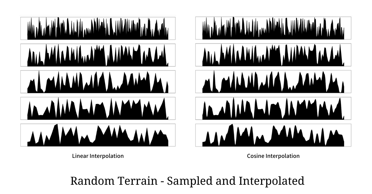
For each interpolation, the 5 plots shown above are sampled for every 1, 2, 3, 4, and 5 points respectively. We can clearly see the plots of Cosine Interpolation are much smoother than Linear Interpolated ones. The technique does a good job over naive implementation but it still does not mimic what we see in the real world. To make things as close to the real-world as possible we use the concept of Superposition.

Superposition Sampled Terrains

Sampling and Interpolation are effective in reducing the spikes and making transitions gradual. The concern with this approach is that sudden changes are not really gone. In order to address this situation, we use the principle of Superposition upon multiple such sampled terrains.

The approach we take here is to generate k such terrains with different sampling frequencies and then perform a normalized weighted sum. This way we get the best of both worlds i.e smoothness from the terrain with the least sampled points and aberrations from the one with the most sampled points.

Now the only piece that remains is choosing the weights. The weights and sampling frequency varies by the power of 2. The number of terrains to be sampled depends on the kind of terrain needed and is to be left for experimentation, but we can assume it to be 6 for most use cases.

The terrain that samples all the points should be given the least weight as it aims to contribute sudden spikes; and as we increase the sampling frequency by the power of 2 we increase the weight by the power of 2 as well. Hence for the first terrain, the scale is 0.03125 where were sample all the points 256, the next terrain is sampled with 128 points and has a scale of 0.0625, and so on till we reach sampled points to be 8 with scale as 1, giving it the highest weight.

Once these terrains are generated we perform a normalized weighted sum and generate the final terrain as shown in the illustration below.

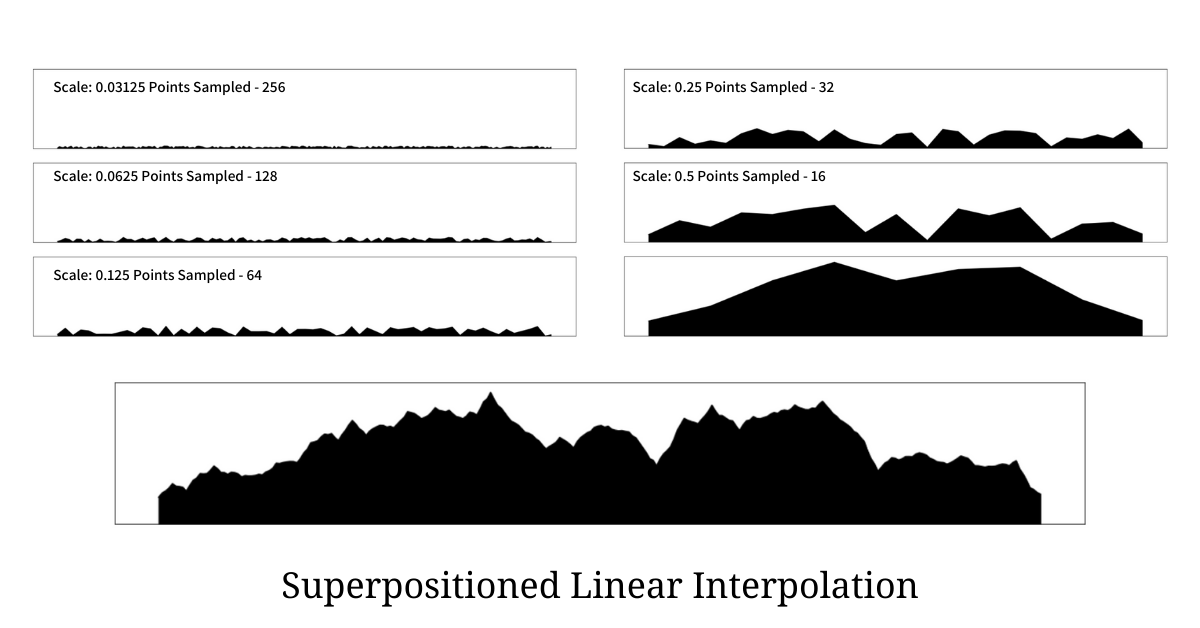
The illustration above shows 6 scaled sampled terrains with different sampling frequencies along with the final super-positioned terrain generated from the procedure. It is very clear that the terrain generated using this procedure is much more closer to the real world terrain than any other we have seen before. Python code that generated the above terrain is as below

def terrain_superpos_linp(naive_terrain, iterations=8) -> List[float]:
    """Using naive terrain `naive_terrain` the function generates
    Linearly Interpolated Superpositioned terrain that looks real world like.
    """
    terrains = []

    # holds the sum of weights for normalization
    weight_sum = 0

    # for every iteration
    for z in range(iterations, 0, -1):
        terrain = []

        # compute the scaling factor (weight)
        weight = 1 / (2 ** (z - 1))

        # compute sampling frequency suggesting every `sample`th
        # point to be picked from the naive terrain.
        sample = 1 << (iterations - z)

        # get the sample points
        sample_points = naive_terrain[::sample]
        
        weight_sum += weight

        for i in range(len(sample_points)):

            # append the current sample point (scaled) to the terrain
            terrain.append(weight * sample_points[i])

            # perform interpolation and add all interpolated values to
            # to the terrain.
            for j in range(sample - 1):
                # compute relative distance from the left point
                mu = (j + 1) / sample

                # compute interpolated point at relative distance of mu
                a = sample_points[i]
                b = sample_points[(i + 1) % len(sample_points)]
                v = linp(a, b, mu)

                # add interpolated point (scaled) to the terrain
                terrain.append(weight * v)

        # append this terrain to list of terrains preparing
        # it to be superpositioned.
        terrains.append(terrain)

    # perform super position and normalization of terrains to
    # get the final terrain
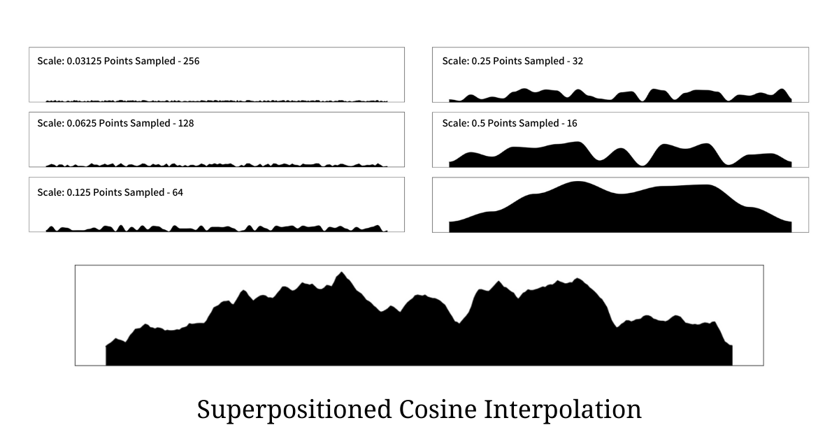
    return [sum(x)/weight_sum for x in zip(*terrains)]

If the terrain to be generated is needed to be smoother then instead of using Linear Interpolation switch to Cosine Interpolation and the resultant terrain will be much smoother and curvier as seen in the illustration below.

This approach is very similar to Perlin Noise that is used for generating multi-dimensional terrains. Ken Perlin was awarded an Academy Award for Technical Achievement for creating the algorithm.

References

• Superposition
• Interpolation Methods
• One Lone Coder - Perlin-like Noise
• IPython notebook with the source code